Decision Tree Basics in SAS and R

Assume we were going to use a decision tree to predict ‘green’ vs. ‘’red” cases (see below- note this plot of the data was actually created in R).

 

We want to use 2 variables say X₁ and X₂ to make a prediction of ‘green’ or ‘red’.  In its simplest form, the decision tree algorithm searches through the values of X₁ and X₂ and finds the values that do the ‘best’ job of ‘splitting’ the cases. For each possible value of X, the algorithm performs a chi-square test. The values that create the best ‘split’ (in SAS Enterprise Miner this is based on a metric called ‘worth’ which is a function of the p-value  associated with the chi-square test  [worth = -log(p-value)]) are chosen. (See below)

 

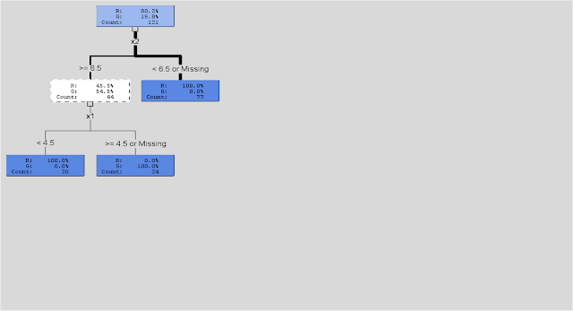
After all of the ‘best’ splits are determined, these values then become rules for distinguishing between cases (in this case ‘green’ vs. ‘red’) What you end up with in the end is a set of ‘rectangles’ defined by a set of ‘rules’ that can be visualized by a ‘tree’ diagram (see visualization from R below). 

 

 (see visualization from SAS Enterpise Miner Below)

But, in SAS Enterprise Miner, the algorithm then goes on to look at new data (validation data) and assesses how well the splitting rules do in terms of predicting or classifying new cases.  If it finds that a ‘smaller’ tree with fewer  variables or fewer splits or rules or ‘branches’ does a better job, it prunes or trims the tree and removes them from the analysis.  In the end, you get a final set of rules that can then be applied algorithmically to predict new cases based on observed values of X₁ and  X₂ (or whatever variables are used by the tree).

In SAS Enterprise Miner, with each split created by the decision tree, a metric for importance based on the Gini impurity index (which is a measure of variability or impurity for categorical data) is calculated. This measures how well the tree distinguishes between cases (again ‘green’ vs. ‘red’ or ‘retained’ vs. ‘non-retained’ in our model) and ultimately how well the model explains whatever it is we are trying to predict.  Overall, if splits based on values of X₂ ‘reduce impurity’ more so than splits based on values of  X₁ , then  X₂ would be considered the ‘best’ or ‘most’ predictive variable. 

The rpart algorithm used in R may differ in some of the specific details, but as discussed in The Elements of Statistical Learning (Hastie, Tibshirani and Friedman (2008)) all decision trees pretty much work the same, fitting the model by recursively partitioning the feature space into rectangular subsets.

 R code for the Decision Tree and Visualizations Above: 

# *------------------------------------------------------------------
# | PROGRAM NAME: R_tree_basic 
# | DATE:4/26/11    
# | CREATED BY: Matt Bogard 
# | PROJECT FILE:P:\R  Code References\Data Mining_R              
# *----------------------------------------------------------------
# | PURPOSE: demo of basic decision tree mechanics               
# |
# *------------------------------------------------------------------
 
rm(list=ls()) # get rid of any existing data 
ls() # view open data sets
 
setwd('/Users/wkuuser/Desktop/R Data Sets') # mac 
setwd("P:\\R  Code References\\R Data") # windows
 
library(rpart) # install rpart decision tree library
 
# *------------------------------------------------------------------
# | get data            
# *-----------------------------------------------------------------
 
dat1 <-  read.csv("basicTree.csv", na.strings=c(".", "NA", "", "?"), encoding="UTF-8")
plot( dat1$x2, dat1$x1, col = dat1$class) # plot data space
 
# fit decision tree
 
(r <- rpart(class ~ x1 + x2, data = dat1)) 
 
plot(r)
text(r)
 
library(rattle) # data mining package
drawTreeNodes(r) # for more detailed tree plot supported by rattle

Created by Pretty R at inside-R.org